Making Network Animations Using NDTV package

Step 1: Load packages

I’ll use statnet, ndtv, and rio packages to make a network gif. statnet and ndtv packages are necessary but you can use other packages instead of rio for loading data. I prefer rio because the command is simple. What we need to do is type ‘import’ as shown in Step 2.

library(statnet)
library(ndtv)
library(rio)

Step 2: Load data

I’ll make a network animation for the formation and dissolution of interstate rivalry from 1987 to 2002 with 5-year intervals (four time points). So, two pieces of information are necessary: 1) a list of rivalries for the given time points (edge list), and 2) a list of countries (node list). The current version of ndtv package doesn’t allow varying numbers of vertices, which means the number of vertices must be the same for all time points. Indeed, some countries newly appeared while others disappeared during the given time period. However, because of the limitation in ndtv, I put all countries existed for the given period in my node list (node.csv).

Additionally, I’ll color the nodes (countries) using their geographical location. For the color of the nodes, I’ll use COW country codes, which are included in ‘vtx1987.csv’ below.

You can download these toy datasets from my github.

riv <- import("C:/Users/bomim/Documents/website-hugo/content/post/toyriv.dta")
vtx <- import("C:/Users/bomim/Documents/website-hugo//content/post/node.csv")
vtx87 <- import("C:/Users/bomim/Documents/website-hugo/content/post/vtx1987.csv")

Step 3: Look at the data

Let’s look at the data we loaded in the previous step. The object ‘riv’ is a list of rivalries (edge list). As shown in the table below, ‘riv’ has four columns: year, stateabb1, stateabb2, and no. Since rivalries are not directed (if Country A is Country B’s rival, then Country B is Country A’s rival as well), the order of stateabb1 and stateabb2 is not important. I’ll use ‘no’ variable to differentiate the four time points from one another.

Because our edge list is made using stateabb (i.e., AAB, AFG, ALB…), our node list must be a list of stateabb.

In terms of the color of nodes, I need more info about the nodes (countries). So, I use the variables in ‘vtx87’. The nodes will be matched using the ‘stateabb’ variable.

head(riv)

##   year stateabb1 stateabb2 no
## 1 1987       AFG       PAK  1
## 2 1992       AFG       PAK  2
## 3 1997       AFG       PAK  3
## 4 2002       AFG       PAK  4
## 5 1997       AFG       TAJ  3
## 6 1997       AFG       UZB  3

head(vtx)

##   stateabb
## 1      AAB
## 2      AFG
## 3      ALB
## 4      ALG
## 5      AND
## 6      ANG

head(vtx87)

##   stateabb ccode        cinc
## 1      AAB    58 0.000002740
## 2      AFG   700 0.001255717
## 3      ALB   339 0.000529850
## 4      ALG   615 0.004066098
## 5      AND   232 0.000000000
## 6      ANG   540 0.001150265

Step 4: Make a list of networks

I use ‘for loop’ to make a list of rivalry networks for four time points. Briefly, I make an empty list (rivlist) first and put each rivalry network for each time point in the list using the for loop.

• More details

The object, ‘nv’, is a numeric value, which shows the total number of countries (the value is 204 in my toy dataset).

Let’s look at the for loop chunk below. This loop will be repeated four times (from 1 to 4). I use ‘no’ for the time points. When i is equal to 1, all rivalries in 1987 are selected (rivi) and two columns from rivi (stateabb1 and stateabb2) would be kept (rivii).

Using the nv (204L), I make an empty network (command: network.initialize). Since there is no direction in rivalries, the option ‘directed’ is FALSE. If your networks of interest are directed (i.e., A thinks B is his/her friend but B doesn’t think like that), then change this option to TRUE. For the network with 204 vertices, I add the vertex names using the command, ‘network.vertex.names’. Now the vertices in the network have their names (stateabb) but still there is no information about ties. The information of ties is loaded from ‘rivii’. The next line is optional. I add info about time points as a vertex attribute (order) to the network. As mentioned above, this sequence is repeated for four time points.

nv <- nrow(vtx)

rivlist <- list()

for(i in 1:4){
  rivi <- subset(riv, riv$no == i)
  rivii<-cbind(rivi$stateabb1, rivi$stateabb2)
  netyr <- network.initialize(nv, directed=FALSE)
  network.vertex.names(x=netyr) <- vtx$stateabb
  netyr[rivii] <- 1
  set.vertex.attribute(x=netyr,attrname="order",val=rep(i,nv))
  rivlist[[i]] <- netyr
}

• Set vertex attribute

As shown in the previous step, we can use ‘set.vertex.attribute’ to add vertex attributes to the network. Following commands are for the color of nodes.

From ‘vtx87’, I add COW country codes for the nodes in the network. This variable is for the color of nodes: red for Americas, orange for Europe, yellow for Africa, green for Middle East, and blue for Asia and Oceania. If you want to color the nodes, you’d better to choose one of the variables which rarely varies over time such as geographical location for countries and gender for individuals. Although ndtv allows us to look at changes in networks such as tie formation and dissolution, it doesn’t allow changes in nodal attributes. For instance, if Country A moved to democracy from non-democracy in 1992 (time point 2), its change cannot be reflected in the network animation.

set.vertex.attribute(rivlist[[1]],names(vtx87),vtx87)

cols1<-vector()
for(i in 1:204){
  ifelse(rivlist[[1]]$val[[i]]$ccode<200, cols1[i] <- "red", 
         ifelse((rivlist[[1]]$val[[i]]$ccode>=200)&(rivlist[[1]]$val[[i]]$ccode<400), cols1[i]<-"orange",
                ifelse((rivlist[[1]]$val[[i]]$ccode>=400)&(rivlist[[1]]$val[[i]]$ccode<630), cols1[i]<-"yellow",
                       ifelse((rivlist[[1]]$val[[i]]$ccode>=630)&(rivlist[[1]]$val[[i]]$ccode<700),cols1[i]<-"green", cols1[i]<-"blue"))))
}

** You can find more commands for data management in R here from my github.

• Make a plot

Let’s look at the rivalry network in 1987 (time point 1). I use the vector of colors (for geographical location) for this plot.

plot(rivlist[[1]], 
     vertex.col=cols1, 
     edge.col="grey50",
     xpd=T)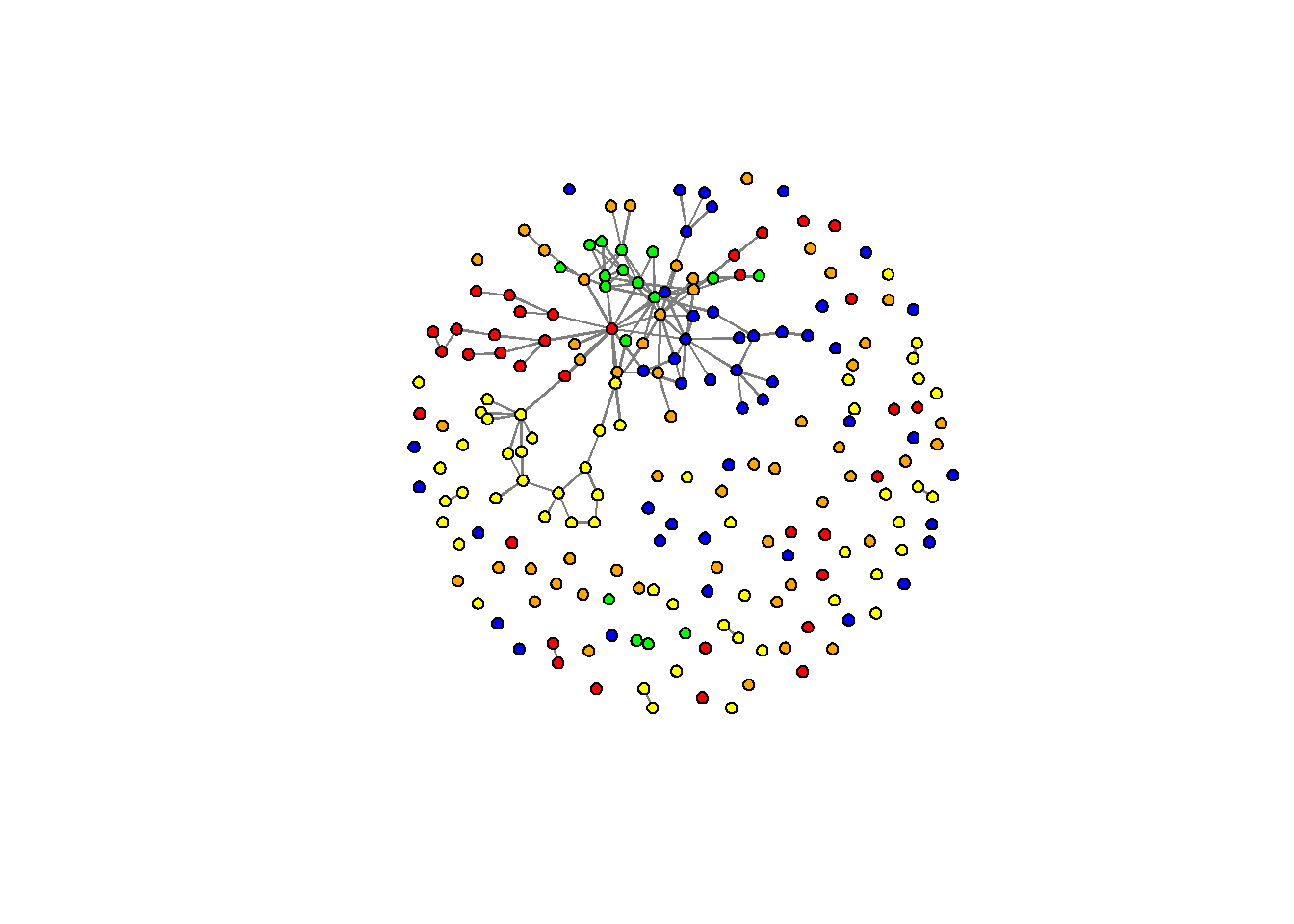

Step 5: Make GIFs!

This is the last step! Make a networkDynamic object using the command ‘networkDynamic’. Before we render an animation, we need one more code here. By using the ‘compute.animation’ command, we can set intervals, animation layout, etc.

rivdyn <- networkDynamic(network.list = rivlist)
rivgif <- compute.animation(rivdyn, 
                            animation.mode = "kamadakawai",
                            verbose = FALSE)

This is the last command. Use the ‘render.d3movie’ command to make a network animation! I add the color vector for this gif!

render.d3movie(rivgif,
               displaylables=FALSE, 
               vertex.col=cols1)

More information about ndtv can be found here.